Image Processing using FFT
The Fast Fourier Transform (FFT) algorithm to calculate discrete Fourier transforms (DFT) is a recent addition to ojAlgo.
The last blog post was about Image Processing (using Singular Value Decomposition, SVD). 2D Fourier transforms can also be used for image processing. Let’s have a look at how to do that.
In image processing, the most common way to represent an image is simply as a matrix of numbers. This is in the spatial domain where the rows and columns map to locations in the image and the numbers/elements to the colour at the respective locations. Sometimes image processing may be inefficient in the spatial domain. Transforming to some other domain may be beneficial.
The FFT is commonly used to transform an image between the spatial and frequency domains. It is the basis for many image filters used to remove noise, sharpen an image, analyse repeating patterns, or extract features. The FFT decomposes an image into sines and cosines of varying amplitudes and phases.
The concrete result of a 2D discrete Fourier transform is a matrix of complex numbers. The dimensions of that matrix is the same as that of the original image. The difference is that now the row/column indices corresponds to (repetition) frequencies rather than positions in the image. The norm of the complex numbers is the amplitude of that particular repetitive pattern. The phase somehow encodes details about the orientation and arrangement in the original image.

In the example program below an image is transformed, processed and then inverse-transformed. The code can be used (by you) with any square image. The first thing the program does is to convert that image to grey scale and resample to ensure that the number of pixels is a power of 2. When that’s done, this is the example’s initial image:
When Fourier transforming an image it is common to also shift the frequencies (rows and columns) so that the zero-frequency is at the centre of the matrix and higher frequencies towards the edges. Low frequencies represent gradual variations in the image; they contain the most information because they determine the overall shape or pattern in the image. High frequencies correspond to abrupt variations in the image; they provide more detail in the image, but also contain more noise. There’s normally a huge difference in amplitude between the low-frequencies (in the center of the image) and the high-frequencies.
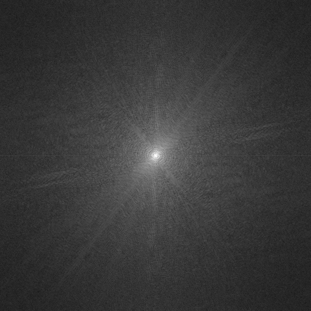
The power spectrum is the squared amplitude of the transform (a matrix where the elements are the complex number norms, squared). This is often plotted in a topology chart or a colour coded image – white for large values and black for small (zero). Due to the huge range of values a base 10 logarithmic scale is used to display the values. These kind of images essentially always show some sort of peak (white spot) in the middle, and then some lighter pattern extending from that, and black/flat edges. Interpreting the exact pattern is for experts.

A simple image filter would define a circle, perhaps based on inspection of the power spectrum, and then treat the values inside or outside that circle differently. A filter that reduce or remove high frequencies (outside the circle) is a called a low-pass filter. A high-pass filter will leave high frequencies unchanged and reduce or remove low frequencies (inside the circle). A low-pass filter will remove detail and noise, as in the example here.
The Code
ImageProcessingFFT.javaimport java.io.File;
import java.io.IOException;
import org.ojalgo.OjAlgoUtils;
import org.ojalgo.data.image.ImageData;
import org.ojalgo.function.constant.PrimitiveMath;
import org.ojalgo.matrix.store.GenericStore;
import org.ojalgo.matrix.store.PhysicalStore;
import org.ojalgo.netio.BasicLogger;
import org.ojalgo.scalar.ComplexNumber;
import org.ojalgo.structure.Transformation2D;
/**
* Basic image processing using the FFT.
* <p>
* Demonstrates how to transform an image to the frequency domain, modify it, and transform it back.
* <p>
* In addition this program shows how to create an image in the frequency domain.
*
* @see https://www.ojalgo.org/2023/12/image-processing-using-fft/
*/
public class ImageProcessingFFT {
static final File BASE_DIR = new File("/Users/apete/Developer/data/fft/");
/**
* Reducing (removing) the image's low-frequency components; a hight-pass filter.
* <p>
* The distance is expressed in percentage of the radius of the largest circle that fits within the image
* – it'll be between 0.0 and 100.0. (Actually, on the diagonal of a square image it will go up to
* 141.42.) Try changing the filter's radius or the multiplier.
*/
static final Transformation2D<ComplexNumber> HIGH_PASS_FILTER = ImageData
.newTransformation((distance, element) -> distance <= 1.0 ? element.multiply(0.2) : element);
/**
* Reducing (removing) the image's high-frequency components; a low-pass filter.
*
* @see #HIGH_PASS_FILTER
*/
static final Transformation2D<ComplexNumber> LOW_PASS_FILTER = ImageData
.newTransformation((distance, element) -> distance >= 1.0 ? element.multiply(0.2) : element);
public static void main(final String[] args) throws IOException {
BasicLogger.debug();
BasicLogger.debug(ImageProcessingFFT.class);
BasicLogger.debug(OjAlgoUtils.getTitle());
BasicLogger.debug(OjAlgoUtils.getDate());
BasicLogger.debug();
/*
* Read any image file (supported by java.awt.image.BufferedImage) and convert it to a grey scale
* image. We assume it's a square image, and resample it to 1024x1024 pixels.
*/
int dim = 1024;
ImageData initialImage = ImageData.read(BASE_DIR, "pexels-any-lane-5946095.jpg").convertToGreyScale().resample(dim, dim);
/*
* Write the initial, grey scale, image to disk.
*/
initialImage.writeTo(BASE_DIR, "initial.png");
/*
* Perform the 2D discrete Fourier transform, and shift the frequencies so that the zero-frequency
* components are in the centre of the image.
*/
PhysicalStore<ComplexNumber> transformed = initialImage.toFrequencyDomain();
/*
* Create an image of the squared magnitudes of the complex numbers in the frequency domain. This is
* the power spectrum of the image.
*/
ImageData.ofPowerSpectrum(transformed).writeTo(BASE_DIR, "powers.png");
/*
* Apply a filter to the frequency domain representation of the image. Here we use a low-pass filter
* to remove the high-frequency components. You can swap the filter to a high-pass filter to remove
* the low-frequency components, or you can create your own filter.
*/
transformed.modifyAny(LOW_PASS_FILTER);
/*
* Write the processed image to disk.
*/
ImageData.fromFrequencyDomain(transformed).writeTo(BASE_DIR, "processed.png");
/*
* It is possible to construct an image in the frequency domain representation. Here we create an
* image by setting a couple of specific values. Try changing the values, the location of the values
* or adding more values.
*/
GenericStore<ComplexNumber> frequencyDomain = GenericStore.C128.make(dim, dim);
/*
* With dim = 1024, the theoretical centre of the image is at (511.5, 511.5). Set values close to the
* centre. Otherwise you wont see the pattern in the image.
*/
/*
* The forward FFT is not scaled, but the inverse is. So you need to scale the values you set here.
* That's why the values are so large.
*/
frequencyDomain.set(512, 506, ComplexNumber.of(128 * dim * dim, 64 * dim * dim));
frequencyDomain.set(508, 514, ComplexNumber.makePolar(255 * dim * dim, PrimitiveMath.HALF_PI));
ImageData.fromFrequencyDomain(frequencyDomain).writeTo(BASE_DIR, "constructed.png");
}
}

It is possible to construct an image by defining a combination of repetitive patterns (sines and cosines) in the frequency domain. This image was generated by the example code by setting 2 elements in a 1024 by 1024 frequency domain matrix, and the inverse-transforming that to spatial (normal image) domain. Try changing the values, the location of the values or adding more values.
- ← Previous
Image Processing using Singular Value Decomposition - Next →
1BRC using ojAlgo