Generalized AutoRegressive Conditional Heteroscedasticity
What is a Generalized AutoRegressive Conditional Heteroscedasticity (GARCH) process?
That’s a long fancy name for something that’s actually relatively simple. The overall context is time series analysis. Let’s sort out the terminology…
Scedasticity
Scedasticity (or skedasticity) is the distribution of error terms (of some random variable). If the variance (and standard deviation) of the error term distribution is constant, we have homoscedasticity. If it’s varying with some kind of pattern we instead have heteroscedasticity. This is what GARCH models are used for – to model time series (financial markets) with turbulent periods of higher volatility than otherwise.
Conditional
In statistics conditional means that you already know something. Conditional probability is the probability of an event occurring, given that another event has already occurred. The concept of conditional probability is primarily related to Bayes’ theorem.
Stationary
Stationary simply means that it doesn’t move or change. A stationary process always has the same mean/expected value. A series of stock prices or index values is not stationary. To use a GARCH model it has to be transformed. Instead of studying the actual values, look at the increments and make those independent of (relative to) the current value (look at the log differences). That’s done with essentially any/all financial time series analysis. GARCH models are used on stationary processes. What changes is the magnitude of the temporary/local errors. It is because we have observed some previous values/errors (conditionality) we can calculate the current expected magnitude of the errors.
AutoRegressive
An autoregressive (regressive on itself) model is when a value from a time series can be expressed as a function of previous values.
AutoRegressive Conditional Heteroscedasticity
An AutoRegressive Conditional Heteroskedasticity (ARCH) model is a statistical model for the variance of a time series, that describe the variance of the current/next error term as a function of the actual (previous) error terms.
GARCH – Generalized AutoRegressive Conditional Heteroscedasticity
The ARCH model refers to a specific formula:

https://en.wikipedia.org/wiki/Autoregressive_conditional_heteroskedasticity
The term “AutoRegressive Conditional Heteroscedasticity” could refer to something much more general than that, but ARCH or ARCH(q) refers to that formula and nothing else. Generalized ARCH, GARCH or GARCH(p, q) also refers to a specific formula:

https://en.wikipedia.org/wiki/Autoregressive_conditional_heteroskedasticity
In fact it’s not that much of a generalisation. Instead of just a weighted sum of past squared errors, there is also a weighted sum of past variances. Since variance is estimated as the average squared error there is an obvious connection between the ARCH and GARCH formulas. In fact an ARCH(∞) model is equivalent to GARCH(1, 1).
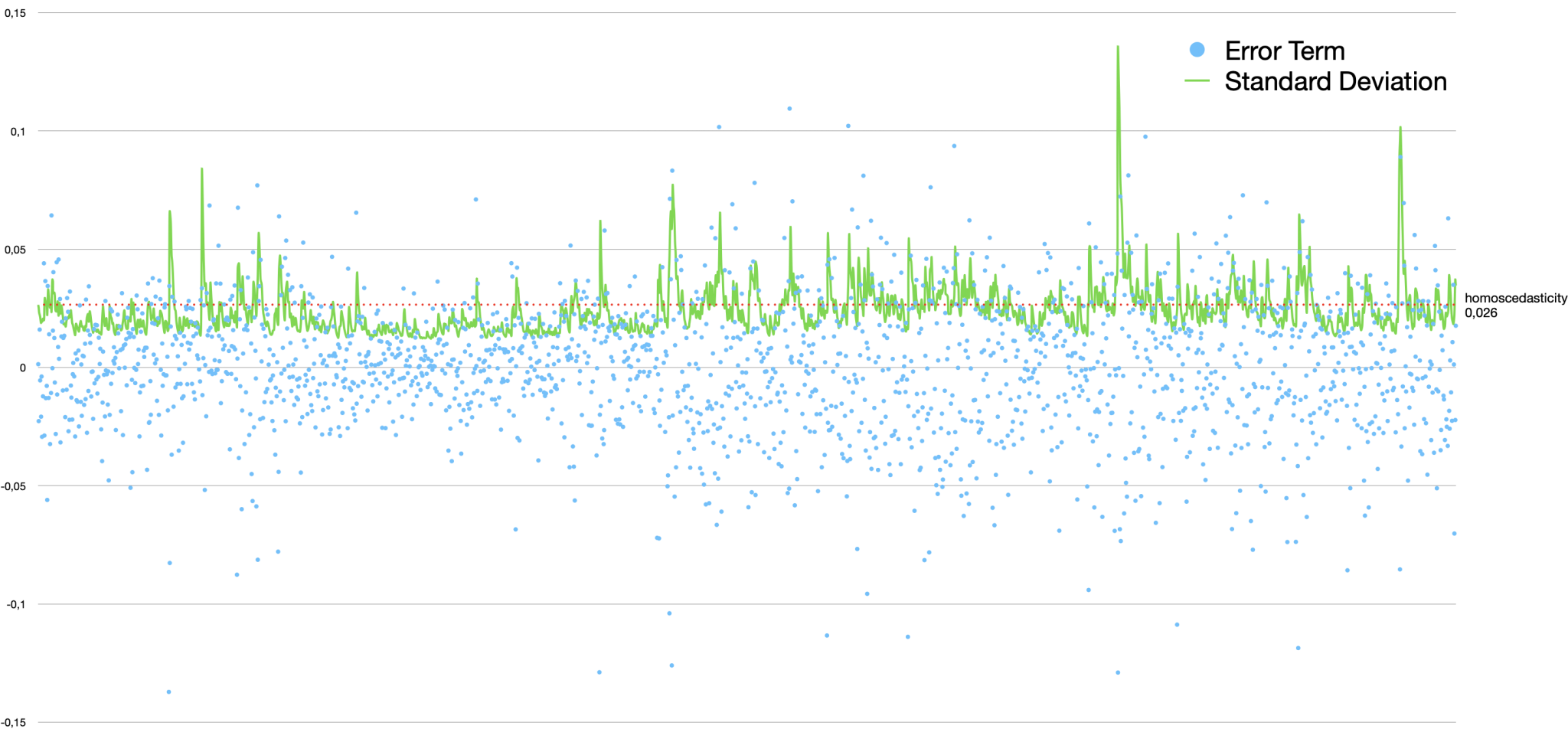
GARCH(2,3) model of the N225 index (57 years weekly data)
Example Code
TimeSeriesGARCH.javaimport java.io.File;
import java.io.IOException;
import java.time.LocalDate;
import org.ojalgo.OjAlgoUtils;
import org.ojalgo.data.domain.finance.series.DataSource;
import org.ojalgo.data.domain.finance.series.FinanceDataReader;
import org.ojalgo.data.domain.finance.series.YahooParser;
import org.ojalgo.data.domain.finance.series.YahooParser.Data;
import org.ojalgo.matrix.store.R032Store;
import org.ojalgo.netio.ASCII;
import org.ojalgo.netio.BasicLogger;
import org.ojalgo.netio.TextLineWriter;
import org.ojalgo.netio.TextLineWriter.CSVLineBuilder;
import org.ojalgo.random.SampleSet;
import org.ojalgo.random.process.RandomProcess.SimulationResults;
import org.ojalgo.random.process.StationaryNormalProcess;
import org.ojalgo.random.scedasticity.GARCH;
import org.ojalgo.series.BasicSeries;
import org.ojalgo.series.primitive.CoordinatedSet;
import org.ojalgo.series.primitive.PrimitiveSeries;
import org.ojalgo.type.CalendarDateUnit;
import org.ojalgo.type.PrimitiveNumber;
import org.ojalgo.type.StandardType;
/**
* Example use of GARCH models, and in addition some general time series handling.
*
* @see https://www.ojalgo.org/2022/07/generalized-autoregressive-conditional-heteroscedasticity/
*/
public abstract class TimeSeriesGARCH {
/**
* A file containing historical data for the Nikkei 225 index, downloaded from Yahoo Finance.
*
* @see https://finance.yahoo.com/quote/^N225/history
*/
static final File N225 = new File("/Users/apete/Developer/data/finance/^N225.csv");
/**
* Where to write output data for the chart.
*/
static final File OUTPUT = new File("/Users/apete/Developer/data/finance/output.csv");
/**
* A file containing historical data for the Russell 2000 index, downloaded from Yahoo Finance.
*
* @see https://finance.yahoo.com/quote/^RUT/history
*/
static final File RUT = new File("/Users/apete/Developer/data/finance/^RUT.csv");
public static void main(final String... args) {
BasicLogger.debug();
BasicLogger.debug(TimeSeriesGARCH.class);
BasicLogger.debug(OjAlgoUtils.getTitle());
BasicLogger.debug(OjAlgoUtils.getDate());
BasicLogger.debug();
FinanceDataReader<Data> readerN225 = FinanceDataReader.of(N225, YahooParser.INSTANCE);
BasicSeries<LocalDate, PrimitiveNumber> seriesN225 = readerN225.getPriceSeries();
BasicLogger.debug("N225: {}", seriesN225.toString());
FinanceDataReader<Data> readerRUT = FinanceDataReader.of(RUT, YahooParser.INSTANCE);
BasicSeries<LocalDate, PrimitiveNumber> seriesRUT = readerRUT.getPriceSeries();
BasicLogger.debug("RUT: {}", seriesRUT.toString());
BasicLogger.debug();
/*
* If you want to calculate something like correlations between a set of series they need to be
* coordinated – the same start, finish and sampling frequency, as well as no missing values.
*/
CoordinatedSet<LocalDate> coordinatedDaily = DataSource.coordinated(CalendarDateUnit.DAY).add(readerN225).add(readerRUT).get();
BasicLogger.debug("Coordinated daily : {}", coordinatedDaily);
/*
* We have 1 value per day, but also know that we're missing data for weekends, holidays and such
* (which need to be filled-in). Could be a good idea to instead coordinate weekly data.
*/
CoordinatedSet<LocalDate> coordinatedWeekly = DataSource.coordinated(CalendarDateUnit.WEEK).add(readerN225).add(readerRUT).get();
BasicLogger.debug("Coordinated weekly : {}", coordinatedWeekly);
/*
* Note that we don't feed the coordinator series, but something that can provide series. In this case
* it's file readers/parsers, but it could just as well be something that calls web services, queries
* a database or whatever. A coordinated data source will populate itself (lazily) on request, and
* then clean up / reset itself using a timer.
*/
CoordinatedSet<LocalDate> coordinatedMonthly = DataSource.coordinated(CalendarDateUnit.MONTH).add(readerN225).add(readerRUT).get();
BasicLogger.debug("Coordinated monthly : {}", coordinatedMonthly);
CoordinatedSet<LocalDate> coordinatedAnnually = DataSource.coordinated(CalendarDateUnit.YEAR).add(readerN225).add(readerRUT).get();
BasicLogger.debug("Coordinated annually: {}", coordinatedAnnually);
BasicLogger.debug();
/*
* Once we have a CoordinatedSet we can easily calculate the correlation coefficients.
*/
R032Store correlations = coordinatedWeekly.log().differences().getCorrelations(R032Store.FACTORY);
BasicLogger.debugMatrix("Correlations", correlations);
/*
* That was a bit of a detour. Now let's focus on just one series, and the volatility of that index.
*/
PrimitiveSeries logDifferences = seriesN225.resample(DataSource.FRIDAY_OF_WEEK).asPrimitive().log().differences();
SampleSet logDifferenceStatistics = SampleSet.wrap(logDifferences);
BasicLogger.debug("Log difference statistics: {}", logDifferenceStatistics.toString());
PrimitiveSeries errorTerms = logDifferences.subtract(logDifferenceStatistics.getMean());
SampleSet errorTermStatistics = SampleSet.wrap(errorTerms);
BasicLogger.debug("Error term statistics: {}", errorTermStatistics.toString());
/*
* If we assume homoscedasticity then the (weekly) variance of the N225 time series is simply the
* variance of the error term sample set. Note also that the variance of the log differences series
* and the error term differences are the same.
*/
BasicLogger.debug();
BasicLogger.debug("Variance");
BasicLogger.debug(1, "of log differences: {}", logDifferenceStatistics.getVariance());
BasicLogger.debug(1, "of error terms : {}", errorTermStatistics.getVariance());
/*
* Any/all financial markets experience periods of turbulence with higher volatility than otherwise.
* To model that we cannot simply have 1 fixed number to describe the volatility of a time series
* spanning almost 60 years. We need something else.
*/
GARCH model = GARCH.estimate(errorTerms, 2, 3);
/*
* GARCH model with 2 lagged variance values and 3 squared error terms
*/
try (TextLineWriter writer = TextLineWriter.of(OUTPUT)) {
// CSV line builder - to help write CSV files
CSVLineBuilder lineBuilder = writer.newCSVLineBuilder(ASCII.HT);
lineBuilder.append("Day").append("Error Term").append("Standard Deviation").write();
/*
* Looping through the error term series. For each item update the GARCH model and write the error
* term and the estimated standard deviation to file. The contents of that file is then used to
* generate the chart in the blog post.
*/
for (int i = 0; i < errorTerms.size(); i++) {
double standardDeviation = model.getStandardDeviation(); // estimated std dev
double value = errorTerms.value(i); // actual value/error (the mean is 0.0)
lineBuilder.append(i).append(value).append(standardDeviation).write();
model.update(value); // update model with actual value
}
} catch (IOException cause) {
throw new RuntimeException(cause);
}
/*
* Presumably the main benefit of using GARCH models is to get a better estimate of current (near
* future) volatility.
*/
/*
* We used weekly values. To annualize volatility it needs to be scaled.
*/
double annualizer = Math.sqrt(52);
BasicLogger.debug();
BasicLogger.debug("Volatility (annualized)");
BasicLogger.debug(1, "constant (homoscedasticity): {}", StandardType.PERCENT.format(annualizer * errorTermStatistics.getStandardDeviation()));
BasicLogger.debug(1, "of GARCH model (current/latest value): {}", StandardType.PERCENT.format(annualizer * model.getStandardDeviation()));
/*
* We can also use the GARCH model to simulate future scenarios.
*/
int numberOfScenarios = 100;
int numberOfProcessSteps = 52;
double processStepSize = 1.0;
/*
* This will simulate 100 scenarios, stepping/incrementing the process 52 times, 1 week at the time.
*/
SimulationResults simulationResults = StationaryNormalProcess.of(model).simulate(numberOfScenarios, numberOfProcessSteps, processStepSize);
}
}
Console Output
class TimeSeriesGARCH
ojAlgo
2022-07-05

N225: First:1965-01-05=1965-01-05: 1257.719971 Last:2022-07-05=2022-07-05: 26423.470703 Size:14141
RUT: First:1987-09-10=1987-09-10: 168.970001 Last:2022-07-01=2022-07-01: 1727.76001 Size:8773

Coordinated daily   : FirstKey=1987-09-10, LastKey=2022-07-01, NumberOfSeries=2, NumberOfSeriesEntries=9046
Coordinated weekly  : FirstKey=1987-09-11, LastKey=2022-07-01, NumberOfSeries=2, NumberOfSeriesEntries=1817
Coordinated monthly : FirstKey=1987-09-30, LastKey=2022-07-31, NumberOfSeries=2, NumberOfSeriesEntries=419
Coordinated annually: FirstKey=1987-12-31, LastKey=2022-12-31, NumberOfSeries=2, NumberOfSeriesEntries=36

Correlations
        1 0.506761
 0.506761        1
Log difference statistics: Sample set Size=2997, Mean=0.0010084690273360743, Var=7.006664819240809E-4, StdDev=0.026470105438476835, Min=-0.27884405377306365, Max=0.15817096723925594
Error term statistics: Sample set Size=2997, Mean=1.2822020166779524E-17, Var=7.006664819240812E-4, StdDev=0.026470105438476842, Min=-0.27985252280039974, Max=0.15716249821191988

Variance
	of log differences: 7.006664819240809E-4
	of error terms    : 7.006664819240812E-4

Volatility (annualized)
	constant (homoscedasticity): 19.09%
	of GARCH model (current/latest value): 21.94%
Further Reading
- https://en.wikipedia.org/wiki/Autoregressive_conditional_heteroskedasticity
- https://online.stat.psu.edu/stat510/lesson/11/11.1
- ← Previous
Optimisation Model File Formats - Next →
LP, QP & MIP on the JVM